Interaction between SuPy and external models
Introduction
SUEWS can be coupled to other models that provide or require forcing data using the SuPy single timestep running mode. We demonstrate this feature with a simple online anthropogenic heat flux model.
Anthropogenic heat flux (\(Q_F\)) is an additional term to the surface energy balance in urban areas associated with human activities (Gabey et al., 2018; Grimmond, 1992; Nie et al., 2014; 2016; Sailor, 2011). In most cities, the largest emission source is from buildings (Hamilton et al., 2009; Iamarino et al., 2011; Sailor, 2011) and is high dependent on outdoor ambient air temperature.
load necessary packages
In [1]:
import supy as sp
import pandas as pd
import numpy as np
import matplotlib.pyplot as plt
import matplotlib.dates as mdates
import seaborn as sns
%matplotlib inline
# produce high-quality figures, which can also be set as one of ['svg', 'pdf', 'retina', 'png']
# 'svg' produces high quality vector figures
from IPython.display import set_matplotlib_formats
set_matplotlib_formats('retina')
print('version info:')
print('supy:',sp.__version__)
print('supy_driver:',sp.__version_driver__)
version info:
supy: 2019.2.8
supy_driver: 2018c5
run SUEWS with default settings
In [2]:
# load sample run dataset
df_state_init, df_forcing = sp.load_SampleData()
df_state_init_def=df_state_init.copy()
# set QF as zero for later comparison
df_forcing_def=df_forcing.copy()
grid=df_state_init_def.index[0]
df_state_init_def.loc[:,'emissionsmethod']=0
df_forcing_def['qf']=0
# run supy
df_output, df_state = sp.run_supy(df_forcing_def, df_state_init_def)
df_output_def = df_output.loc[grid, 'SUEWS']
a simple QF model: QF_simple
model description
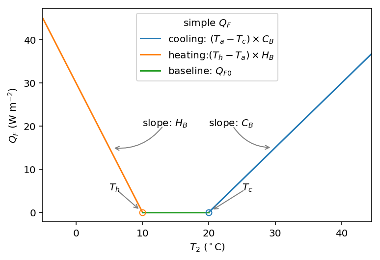
For demonstration purposes we have created a very simple model instead of using the SUEWS \(Q_F\) (Järvi et al. 2011) with feedback from outdoor air temperature. The simple \(Q_F\) model considers only building heating and cooling:
temperature of buildings, \(𝐶_B\) (\(𝐻_B\)) is the building cooling (heating) rate, and \(𝑄_{F0}\) is the baseline anthropogenic heat. The parameters used are: \(𝑇_C\) (\(𝑇_H\)) set as 20 °C (10 °C), \(𝐶_B\) (\(𝐻_B\)) set as 1.5 \(\mathrm{W\ m^{-2}\ K^{-1}}\) (3 \(\mathrm{W\ m^{-2}\ K^{-1}}\)) and \(Q_{F0}\) is set as 0 \(\mathrm{W\ m^{-2}}\), implying other building activities (e.g. lightning, water heating, computers) are zero and therefore do not change the temperature or change with temperature.
implementation
In [3]:
def QF_simple(T2):
    qf_cooling = (T2-20)*5 if T2 > 20 else 0
    qf_heating = (10-T2)*10 if T2 < 10 else 0
    qf_res = np.max([qf_heating, qf_cooling])*0.3
    return qf_res
In [4]:
ser_temp = pd.Series(
    np.arange(-5, 45, 0.5), index=np.arange(-5, 45, 0.5)).rename('temp_C')
ser_qf_heating = ser_temp.loc[-5:10].map(QF_simple).rename(
    r'heating:$(T_h-T_a) \times H_B$')
ser_qf_cooling = ser_temp.loc[20:45].map(QF_simple).rename(
    r'cooling: $(T_a-T_c) \times C_B$')
ser_qf_zero = ser_temp.loc[10:20].map(QF_simple).rename('baseline: $Q_{F0}$')
df_temp_qf = pd.concat([
    ser_temp,
    ser_qf_cooling,
    ser_qf_heating,
    ser_qf_zero,
],
                       axis=1).set_index('temp_C')
ax_qf_func = df_temp_qf.plot()
ax_qf_func.set_xlabel('$T_2$ ($^\circ$C)')
ax_qf_func.set_ylabel('$Q_F$ ($ \mathrm{W \ m^{-2}}$)')
ax_qf_func.legend(title='simple $Q_F$')
ax_qf_func.annotate("$T_c$",
                xy=(20, 0), xycoords='data',
                xytext=(25, 5), textcoords='data',
                arrowprops=dict(arrowstyle="->", #linestyle="dashed",
                                color="0.5",
                                shrinkA=5, shrinkB=5,
                                patchA=None,
                                patchB=None,
                                connectionstyle='arc3',
                                ),
                )

ax_qf_func.annotate("$T_h$",
                xy=(10, 0), xycoords='data',
                xytext=(5, 5), textcoords='data',
                arrowprops=dict(arrowstyle="->", #linestyle="dashed",
                                color="0.5",
                                shrinkA=5, shrinkB=5,
                                patchA=None,
                                patchB=None,
                                connectionstyle='arc3',
                                ),
                )
ax_qf_func.annotate("slope: $C_B$",
                xy=(30, QF_simple(30)), xycoords='data',
                xytext=(20, 20), textcoords='data',
                arrowprops=dict(arrowstyle="->", #linestyle="dashed",
                                color="0.5",
                                shrinkA=5, shrinkB=5,
                                patchA=None,
                                patchB=None,
                                connectionstyle='arc3, rad=0.3',
                                ),
                )
ax_qf_func.annotate("slope: $H_B$",
                xy=(5, QF_simple(5)), xycoords='data',
                xytext=(10, 20), textcoords='data',
                arrowprops=dict(arrowstyle="->", #linestyle="dashed",
                                color="0.5",
                                shrinkA=5, shrinkB=5,
                                patchA=None,
                                patchB=None,
                                connectionstyle='arc3, rad=-0.3',
                                ),
                )
ax_qf_func.plot(10,0,'o',color='C1',fillstyle='none')
_=ax_qf_func.plot(20,0,'o',color='C0',fillstyle='none')
communication between supy and QF_simple
construct a new coupled function
The coupling between the simple \(Q_F\) model and SuPy is done via
the low-level function suews_cal_tstep, which is an interface
function in charge of communications between SuPy frontend and the
calculation kernel. By setting SuPy to receive external \(Q_F\) as
forcing, at each timestep, the simple \(Q_F\) model is driven by the
SuPy output \(T_2\) and provides SuPy with \(Q_F\), which thus
forms a two-way coupled loop.
In [5]:
# load extra low-level functions from supy to construct interactive functions
from supy.supy_post import pack_df_output, pack_df_state
from supy.supy_run import suews_cal_tstep, pack_grid_dict


def run_supy_qf(df_forcing_test, df_state_init_test):
    grid = df_state_init_test.index[0]
    df_state_init_test.loc[grid, 'emissionsmethod'] = 0

    df_forcing_test = df_forcing_test\
        .assign(
            metforcingdata_grid=0,
            ts5mindata_ir=0,
        )\
        .rename(
            # remanae is a workaround to resolve naming inconsistency between
            # suews fortran code interface and input forcing file hearders
            columns={
                '%' + 'iy': 'iy',
                'id': 'id',
                'it': 'it',
                'imin': 'imin',
                'qn': 'qn1_obs',
                'qh': 'qh_obs',
                'qe': 'qe',
                'qs': 'qs_obs',
                'qf': 'qf_obs',
                'U': 'avu1',
                'RH': 'avrh',
                'Tair': 'temp_c',
                'pres': 'press_hpa',
                'rain': 'precip',
                'kdown': 'avkdn',
                'snow': 'snow_obs',
                'ldown': 'ldown_obs',
                'fcld': 'fcld_obs',
                'Wuh': 'wu_m3',
                'xsmd': 'xsmd',
                'lai': 'lai_obs',
                'kdiff': 'kdiff',
                'kdir': 'kdir',
                'wdir': 'wdir',
            }
        )

    t2_ext = df_forcing_test.iloc[0].temp_c
    qf_ext = QF_simple(t2_ext)

    # initialise dicts for holding results
    dict_state = {}
    dict_output = {}

    # starting tstep
    t_start = df_forcing_test.index[0]
    # convert df to dict with `itertuples` for better performance
    dict_forcing = {
        row.Index: row._asdict()
        for row in df_forcing_test.itertuples()
    }
    # dict_state is used to save model states for later use
    dict_state = {(t_start, grid): pack_grid_dict(series_state_init)
                  for grid, series_state_init in df_state_init_test.iterrows()}

    # just use a single grid run for the test coupling
    for tstep in df_forcing_test.index:
        # load met forcing at `tstep`
        met_forcing_tstep = dict_forcing[tstep]
        # inject `qf_ext` to `met_forcing_tstep`
        met_forcing_tstep['qf_obs'] = qf_ext

        # update model state
        dict_state_start = dict_state[(tstep, grid)]

        dict_state_end, dict_output_tstep = suews_cal_tstep(
            dict_state_start, met_forcing_tstep)
        t2_ext = dict_output_tstep['dataoutlinesuews'][-3]
        qf_ext = QF_simple(t2_ext)

        dict_output.update({(tstep, grid): dict_output_tstep})
        dict_state.update({(tstep + 1, grid): dict_state_end})

    # pack results as easier DataFrames
    df_output_test = pack_df_output(dict_output).swaplevel(0, 1)
    df_state_test = pack_df_state(dict_state).swaplevel(0, 1)
    return df_output_test.loc[grid, 'SUEWS'], df_state_test
simulations for summer and winter months
The simulation using SuPy coupled is performed for London 2012. The data analysed are a summer (July) and a winter (December) month. Initially \(Q_F\) is 0 \(\mathrm{W\ m^{-2}}\) the \(T_2\) is determined and used to determine \(Q_{F[1]}\) which in turn modifies \(T_{2[1]}\) and therefore modifies \(Q_{F[2]}\) and the diagnosed \(T_{2[2]}\).
spinup run (January to June) for summer simulation
In [6]:
df_output_june, df_state_jul = sp.run_supy(
    df_forcing.loc[:'2012 6'], df_state_init)
df_state_jul_init = df_state_jul.reset_index('datetime', drop=True).iloc[[-1]]
spinup run (July to October) for winter simulation
In [7]:
df_output_oct, df_state_dec = sp.run_supy(
    df_forcing.loc['2012 7':'2012 11'], df_state_jul_init)
df_state_dec_init = df_state_dec.reset_index('datetime', drop=True).iloc[[-1]]
coupled simulation
In [8]:
df_output_test_summer, df_state_summer_test = run_supy_qf(
    df_forcing.loc['2012 7'], df_state_jul_init.copy())
df_output_test_winter, df_state_winter_test = run_supy_qf(
    df_forcing.loc['2012 12'], df_state_dec_init.copy())
examine the results
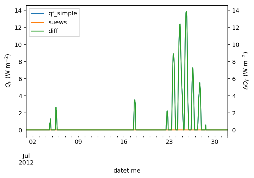
sumer
In [9]:
var = 'QF'
var_label = '$Q_F$ ($ \mathrm{W \ m^{-2}}$)'
var_label_right = '$\Delta Q_F$ ($ \mathrm{W \ m^{-2}}$)'
period = '2012 7'
df_test = df_output_test_summer
y1 = df_test.loc[period, var].rename('qf_simple')
y2 = df_output_def.loc[period, var].rename('suews')
y3 = (y1-y2).rename('diff')
df_plot = pd.concat([y1, y2, y3], axis=1)
ax = df_plot.plot(secondary_y='diff')
ax.set_ylabel(var_label)
# sns.lmplot(data=df_plot,x='qf_simple',y='diff')
ax.right_ax.set_ylabel(var_label_right)
lines = ax.get_lines() + ax.right_ax.get_lines()
ax.legend(lines, [l.get_label() for l in lines], loc='best')
Out[9]:
<matplotlib.legend.Legend at 0x130455e48>
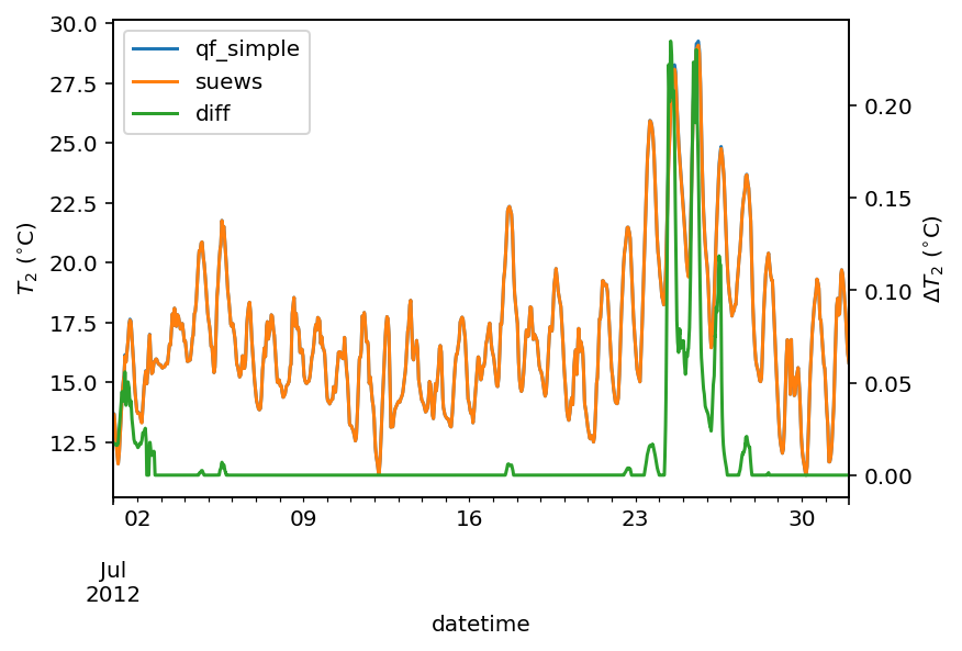
In [10]:
var = 'T2'
var_label = '$T_2$ ($^{\circ}$C)'
var_label_right = '$\Delta T_2$ ($^{\circ}$C)'
period = '2012 7'
df_test = df_output_test_summer
y1 = df_test.loc[period, var].rename('qf_simple')
y2 = df_output_def.loc[period, var].rename('suews')
y3 = (y1-y2).rename('diff')
df_plot = pd.concat([y1, y2, y3], axis=1)
ax = df_plot.plot(secondary_y='diff')
ax.set_ylabel(var_label)
ax.right_ax.set_ylabel(var_label_right)
lines = ax.get_lines() + ax.right_ax.get_lines()
ax.legend(lines, [l.get_label() for l in lines], loc='best')
Out[10]:
<matplotlib.legend.Legend at 0x1303b0208>
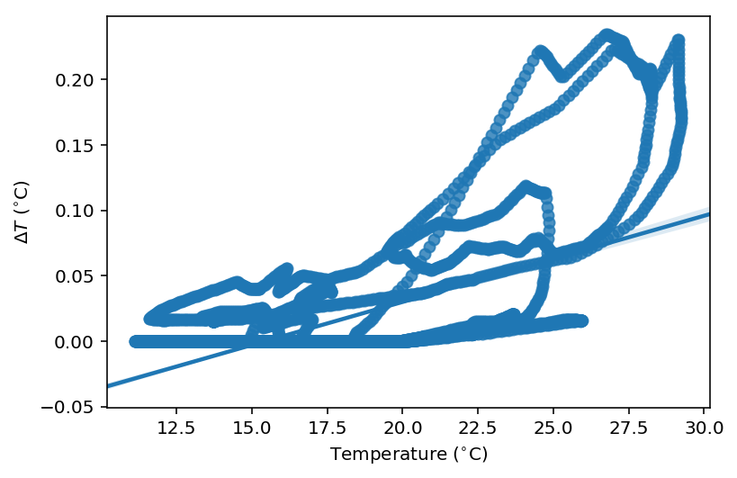
In [11]:
ax_t2diff = sns.regplot(
    data=df_plot.loc[df_plot['diff'] != 0], x='qf_simple', y='diff')
ax_t2diff.set_ylabel('$\Delta T$ ($^{\circ}$C)')
_=ax_t2diff.set_xlabel('Temperature ($^{\circ}$C)')
winter
In [12]:
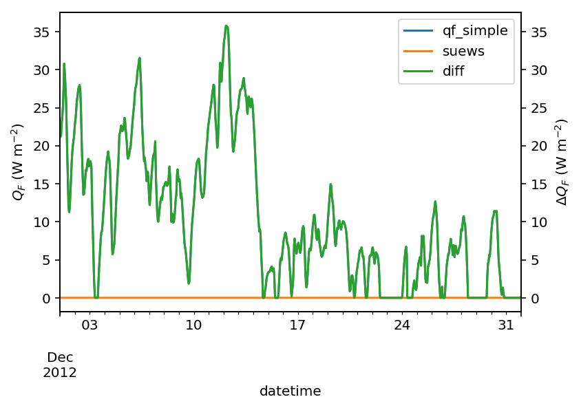
var = 'QF'
var_label = '$Q_F$ ($ \mathrm{W \ m^{-2}}$)'
var_label_right = '$\Delta Q_F$ ($ \mathrm{W \ m^{-2}}$)'
period = '2012 12'
df_test = df_output_test_winter
y1 = df_test.loc[period, var].rename('qf_simple')
y2 = df_output_def.loc[period, var].rename('suews')
y3 = (y1-y2).rename('diff')
df_plot = pd.concat([y1, y2, y3], axis=1)
ax = df_plot.plot(secondary_y='diff')
ax.set_ylabel(var_label)
# sns.lmplot(data=df_plot,x='qf_simple',y='diff')
ax.right_ax.set_ylabel(var_label_right)
lines = ax.get_lines() + ax.right_ax.get_lines()
ax.legend(lines, [l.get_label() for l in lines], loc='best')
Out[12]:
<matplotlib.legend.Legend at 0x10cdea828>
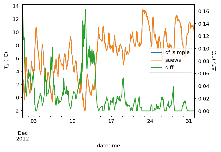
In [13]:
var = 'T2'
var_label = '$T_2$ ($^{\circ}$C)'
var_label_right = '$\Delta T_2$ ($^{\circ}$C)'
period = '2012 12'
df_test = df_output_test_winter
y1 = df_test.loc[period, var].rename('qf_simple')
y2 = df_output_def.loc[period, var].rename('suews')
y3 = (y1-y2).rename('diff')
df_plot = pd.concat([y1, y2, y3], axis=1)
ax = df_plot.plot(secondary_y='diff')
ax.set_ylabel(var_label)
ax.right_ax.set_ylabel(var_label_right)
lines = ax.get_lines() + ax.right_ax.get_lines()
ax.legend(lines, [l.get_label() for l in lines], loc='center right')
Out[13]:
<matplotlib.legend.Legend at 0x141a85940>
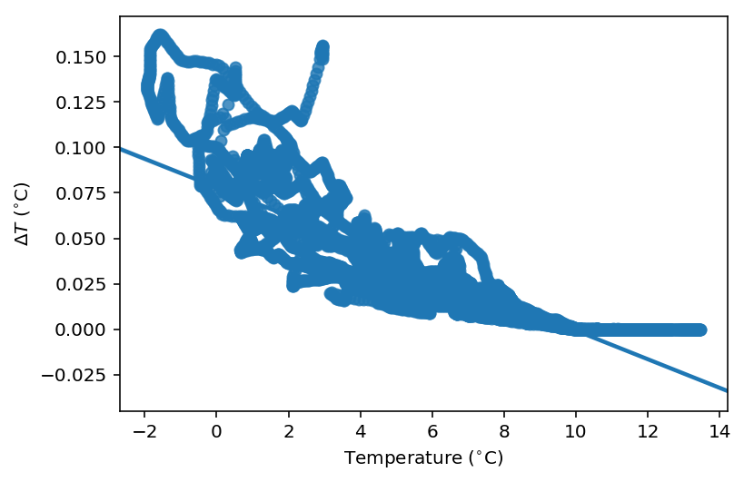
In [14]:
%config InlineBackend.figure_format='retina'
ax_t2diff = sns.regplot(
    data=df_plot.loc[df_plot['diff'] > 0],
    x='qf_simple', y='diff')
ax_t2diff.set_ylabel('$\Delta T$ ($^{\circ}$C)')
ax_t2diff.set_xlabel('Temperature ($^{\circ}$C)')
Out[14]:
Text(0.5, 0, 'Temperature ($^{\\circ}$C)')
comparison in \(\Delta Q_F\)-\(\Delta T2\) feedback between summer and winter
In [15]:
# set_matplotlib_formats('retina')
df_diff_summer = (df_output_test_summer -
                  df_output_def).dropna(how='all', axis=0)
df_diff_winter = (df_output_test_winter -
                  df_output_def).dropna(how='all', axis=0)
In [16]:
# set_matplotlib_formats('retina')
df_diff_season = pd.concat([
    df_diff_winter.assign(season='winter'),
    df_diff_summer.assign(season='summer'),
]).loc[:, ['season', 'QF', 'T2']]
g = sns.lmplot(
    data=df_diff_season,
    x='QF',
    y='T2',
#     col='season',
    hue='season',
    height=4,
    truncate=False,
    markers='o',
    legend_out=False,
    scatter_kws={
#         'facecolor':'none',
        's':1,
        'zorder':0,
        'alpha':0.8,
    },
    line_kws={
#         'facecolor':'none',
        'zorder':6,
        'linestyle':'--'
    },
)
g.set_axis_labels(
    '$\Delta Q_F$ ($ \mathrm{W \ m^{-2}}$)',
    '$\Delta T_2$ ($^{\circ}$C)',
)
g.ax.legend(markerscale=4,title='season')
g.despine(top=False, right=False)
Out[16]:
<seaborn.axisgrid.FacetGrid at 0x13d10d828>
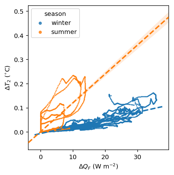
The above figure indicate a positive feedback, as \(Q_F\) is increased there is an elevated \(T_2\) but with different magnitudes. Of particular note is the positive feedback loop under warm air temperatures: the anthropogenic heat emissions increase which in turn elevates the outdoor air temperature causing yet more anthropogenic heat release. Note that London is relatively cool so the enhancement is much less than it would be in warmer cities.