Note
1. This page was generated from docs/source/tutorial/quick-start.ipynb.
Interactive online version:
![]() Slideshow:
Slideshow:
![]()
- Need help? Please let us know in the UMEP Community.
- A good understanding of SUEWS is a prerequisite to the proper use of SuPy.
Quickstart of SuPy
This quickstart demonstrates the essential and simplest workflow of supy in SUEWS simulation:
More advanced use of supy are available in the tutorials
Before we start, we need to load the following necessary packages.
[1]:
import matplotlib.pyplot as plt
import supy as sp
import pandas as pd
import numpy as np
from pathlib import Path

%matplotlib inline
[2]:
sp.show_version()
SuPy versions
-------------
supy: 2020.7.1dev
supy_driver: 2020b1

=================
SYSTEM DEPENDENCY

INSTALLED VERSIONS
------------------
commit           : None
python           : 3.7.3.final.0
python-bits      : 64
OS               : Darwin
OS-release       : 19.5.0
machine          : x86_64
processor        : i386
byteorder        : little
LC_ALL           : None
LANG             : en_US.UTF-8
LOCALE           : en_US.UTF-8

pandas           : 1.0.3
numpy            : 1.17.5
pytz             : 2019.3
dateutil         : 2.8.1
pip              : 19.3.1
setuptools       : 45.1.0.post20200119
Cython           : None
pytest           : 5.3.1
hypothesis       : None
sphinx           : 3.1.1
blosc            : None
feather          : None
xlsxwriter       : None
lxml.etree       : 4.5.0
html5lib         : None
pymysql          : None
psycopg2         : None
jinja2           : 2.10.3
IPython          : 7.11.1
pandas_datareader: None
bs4              : 4.8.2
bottleneck       : None
fastparquet      : None
gcsfs            : None
lxml.etree       : 4.5.0
matplotlib       : 3.1.2
numexpr          : 2.7.1
odfpy            : None
openpyxl         : None
pandas_gbq       : None
pyarrow          : None
pytables         : None
pytest           : 5.3.1
pyxlsb           : None
s3fs             : None
scipy            : 1.4.1
sqlalchemy       : None
tables           : 3.6.1
tabulate         : 0.8.6
xarray           : 0.14.1
xlrd             : None
xlwt             : None
xlsxwriter       : None
numba            : 0.46.0
Load input files
For existing SUEWS users:
First, a path to SUEWS RunControl.nml should be specified, which will direct supy to locate input files.
[3]:
path_runcontrol = Path('../sample_run') / 'RunControl.nml'
[4]:
df_state_init = sp.init_supy(path_runcontrol)
2020-07-05 22:59:45,696 - SuPy - INFO - All cache cleared.
A sample df_state_init looks below (note that .T is used here to produce a nicer tableform view):
[5]:
df_state_init.filter(like='method').T
[5]:
| grid | 1 | |
|---|---|---|
| var | ind_dim | |
| aerodynamicresistancemethod | 0 | 2 |
| basetmethod | 0 | 1 |
| evapmethod | 0 | 2 |
| emissionsmethod | 0 | 2 |
| netradiationmethod | 0 | 3 |
| roughlenheatmethod | 0 | 2 |
| roughlenmommethod | 0 | 2 |
| smdmethod | 0 | 0 |
| stabilitymethod | 0 | 3 |
| storageheatmethod | 0 | 1 |
| waterusemethod | 0 | 0 |
Following the convention of SUEWS, supy loads meteorological forcing (met-forcing) files at the grid level.
[6]:
grid = df_state_init.index[0]
df_forcing = sp.load_forcing_grid(path_runcontrol, grid)
# by default, two years of forcing data are included;
# to save running time for demonstration, we only use one year in this demo
df_forcing=df_forcing.loc['2012'].iloc[1:]
2020-07-05 22:59:47,526 - SuPy - INFO - All cache cleared.
For new users to SUEWS/SuPy:
To ease the input file preparation, a helper function load_SampleData is provided to get the sample input for SuPy simulations
[7]:
df_state_init, df_forcing = sp.load_SampleData()
grid = df_state_init.index[0]
# by default, two years of forcing data are included;
# to save running time for demonstration, we only use one year in this demo
df_forcing=df_forcing.loc['2012'].iloc[1:]
2020-07-05 22:59:50,754 - SuPy - INFO - All cache cleared.
Overview of SuPy input
df_state_init
df_state_init includes model Initial state consisting of:
- surface characteristics (e.g., albedo, emissivity, land cover fractions, etc.; full details refer to SUEWS documentation)
- model configurations (e.g., stability; full details refer to SUEWS documentation)
Detailed description of variables in df_state_init refers to SuPy input
Surface land cover fraction information in the sample input dataset:
[8]:
df_state_init.loc[:,['bldgh','evetreeh','dectreeh']]
[8]:
| var | bldgh | dectreeh | evetreeh |
|---|---|---|---|
| ind_dim | 0 | 0 | 0 |
| grid | |||
| 1 | 22.0 | 13.1 | 13.1 |
[9]:
df_state_init.filter(like='sfr')
[9]:
| var | sfr | ||||||
|---|---|---|---|---|---|---|---|
| ind_dim | (0,) | (1,) | (2,) | (3,) | (4,) | (5,) | (6,) |
| grid | |||||||
| 1 | 0.43 | 0.38 | 0.0 | 0.02 | 0.03 | 0.0 | 0.14 |
df_forcing
df_forcing includes meteorological and other external forcing information.
Detailed description of variables in df_forcing refers to SuPy input.
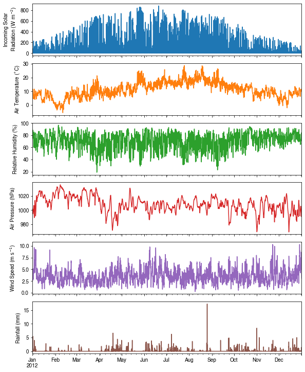
Below is an overview of forcing variables of the sample data set used in the following simulations.
[10]:
list_var_forcing = [
    "kdown",
    "Tair",
    "RH",
    "pres",
    "U",
    "rain",
]
dict_var_label = {
    "kdown": "Incoming Solar\n Radiation ($ \mathrm{W \ m^{-2}}$)",
    "Tair": "Air Temperature ($^{\circ}}$C)",
    "RH": r"Relative Humidity (%)",
    "pres": "Air Pressure (hPa)",
    "rain": "Rainfall (mm)",
    "U": "Wind Speed (m $\mathrm{s^{-1}}$)",
}
df_plot_forcing_x = (
    df_forcing.loc[:, list_var_forcing].copy().shift(-1).dropna(how="any")
)
df_plot_forcing = df_plot_forcing_x.resample("1h").mean()
df_plot_forcing["rain"] = df_plot_forcing_x["rain"].resample("1h").sum()

axes = df_plot_forcing.plot(subplots=True, figsize=(8, 12), legend=False,)
fig = axes[0].figure
fig.tight_layout()
fig.autofmt_xdate(bottom=0.2, rotation=0, ha="center")
for ax, var in zip(axes, list_var_forcing):
    _ = ax.set_ylabel(dict_var_label[var])
Modification of SuPy input
Given pandas.DataFrame is the core data structure of SuPy, all operations, including modification, output, demonstration, etc., on SuPy inputs (df_state_init and df_forcing) can be done using pandas-based functions/methods.
Specifically, for modification, the following operations are essential:
locating data
Data can be located in two ways, namely: 1. by name via `.loc <http://pandas.pydata.org/pandas-docs/stable/user_guide/indexing.html#selection-by-label>`__; 2. by position via `.iloc <http://pandas.pydata.org/pandas-docs/stable/user_guide/indexing.html#selection-by-position>`__.
[11]:
# view the surface fraction variable: `sfr`
df_state_init.loc[:,'sfr']
[11]:
| ind_dim | (0,) | (1,) | (2,) | (3,) | (4,) | (5,) | (6,) |
|---|---|---|---|---|---|---|---|
| grid | |||||||
| 1 | 0.43 | 0.38 | 0.0 | 0.02 | 0.03 | 0.0 | 0.14 |
[12]:
# view the second row of `df_forcing`, which is a pandas Series
df_forcing.iloc[1]
[12]:
iy       2012.000000
id          1.000000
it          0.000000
imin       10.000000
qn       -999.000000
qh       -999.000000
qe       -999.000000
qs       -999.000000
qf       -999.000000
U           5.176667
RH         86.195000
Tair       11.620000
pres     1001.833333
rain        0.000000
kdown       0.173333
snow     -999.000000
ldown    -999.000000
fcld     -999.000000
Wuh         0.000000
xsmd     -999.000000
lai      -999.000000
kdiff    -999.000000
kdir     -999.000000
wdir     -999.000000
isec        0.000000
Name: 2012-01-01 00:10:00, dtype: float64
[13]:
# view a particular position of `df_forcing`, which is a value
df_forcing.iloc[8,9]
[13]:
4.78
setting new values
Setting new values is very straightforward: after locating the variables/data to modify, just set the new values accordingly:
[14]:
# modify surface fractions
df_state_init.loc[:,'sfr']=[.1,.1,.2,.3,.25,.05,0]
# check the updated values
df_state_init.loc[:,'sfr']
[14]:
| ind_dim | (0,) | (1,) | (2,) | (3,) | (4,) | (5,) | (6,) |
|---|---|---|---|---|---|---|---|
| grid | |||||||
| 1 | 0.1 | 0.1 | 0.2 | 0.3 | 0.25 | 0.05 | 0.0 |
Run simulations
Once met-forcing (via df_forcing) and initial conditions (via df_state_init) are loaded in, we call sp.run_supy to conduct a SUEWS simulation, which will return two pandas DataFrames: df_output and df_state.
[15]:
df_output, df_state_final = sp.run_supy(df_forcing, df_state_init)
2020-07-05 22:59:56,659 - SuPy - INFO - ====================
2020-07-05 22:59:56,660 - SuPy - INFO - Simulation period:
2020-07-05 22:59:56,660 - SuPy - INFO -   Start: 2012-01-01 00:05:00
2020-07-05 22:59:56,661 - SuPy - INFO -   End: 2012-12-31 23:55:00
2020-07-05 22:59:56,662 - SuPy - INFO -
2020-07-05 22:59:56,662 - SuPy - INFO - No. of grids: 1
2020-07-05 22:59:56,663 - SuPy - INFO - SuPy is running in serial mode
2020-07-05 23:00:15,586 - SuPy - INFO - Execution time: 18.9 s
2020-07-05 23:00:15,587 - SuPy - INFO - ====================
df_output
df_output is an ensemble output collection of major SUEWS output groups, including:
- SUEWS: the essential SUEWS output variables
- DailyState: variables of daily state information
- snow: snow output variables (effective when
snowuse = 1set indf_state_init)
Detailed description of variables in df_output refers to SuPy output
[16]:
df_output.columns.levels[0]
[16]:
Index(['SUEWS', 'snow', 'RSL', 'SOLWEIG', 'DailyState'], dtype='object', name='group')
df_state_final
df_state_final is a DataFrame for holding:
- all model states if
save_stateis set toTruewhen callingsp.run_supy(supymay run significantly slower for a large simulation); - or, only the final state if
save_stateis set toFalse(the default setting), in which modesupyhas a similar performance as the standalone compiled SUEWS executable.
Entries in df_state_final have the same data structure as df_state_init and can thus be used for other SUEWS simulations starting at the timestamp as in df_state_final.
Detailed description of variables in df_state_final refers to SuPy output
[17]:
df_state_final.T.head()
[17]:
| datetime | 2012-01-01 00:05:00 | 2013-01-01 00:00:00 | |
|---|---|---|---|
| grid | 1 | 1 | |
| var | ind_dim | ||
| ah_min | (0,) | 15.0 | 15.0 |
| (1,) | 15.0 | 15.0 | |
| ah_slope_cooling | (0,) | 2.7 | 2.7 |
| (1,) | 2.7 | 2.7 | |
| ah_slope_heating | (0,) | 2.7 | 2.7 |
Examine results
Thanks to the functionality inherited from pandas and other packages under the PyData stack, compared with the standard SUEWS simulation workflow, supy enables more convenient examination of SUEWS results by statistics calculation, resampling, plotting (and many more).
Ouptut structure
df_output is organised with MultiIndex (grid,timestamp) and (group,varaible) as index and columns, respectively.
[18]:
df_output.head()
[18]:
| group | SUEWS | ... | DailyState | |||||||||||||||||||
|---|---|---|---|---|---|---|---|---|---|---|---|---|---|---|---|---|---|---|---|---|---|---|
| var | Kdown | Kup | Ldown | Lup | Tsurf | QN | QF | QS | QH | QE | ... | DensSnow_Paved | DensSnow_Bldgs | DensSnow_EveTr | DensSnow_DecTr | DensSnow_Grass | DensSnow_BSoil | DensSnow_Water | a1 | a2 | a3 | |
| grid | datetime | |||||||||||||||||||||
| 1 | 2012-01-01 00:05:00 | 0.176667 | 0.021459 | 344.179805 | 371.680316 | 11.607207 | -27.345303 | 40.574001 | -5.886447 | 15.276915 | -7.777741 | ... | NaN | NaN | NaN | NaN | NaN | NaN | NaN | NaN | NaN | NaN |
| 2012-01-01 00:10:00 | 0.173333 | 0.046164 | 344.190048 | 372.637243 | 11.620000 | -28.320026 | 39.724283 | -1.013319 | -22.518257 | -81.748807 | ... | NaN | NaN | NaN | NaN | NaN | NaN | NaN | NaN | NaN | NaN | |
| 2012-01-01 00:15:00 | 0.170000 | 0.045271 | 344.200308 | 372.715137 | 11.635000 | -28.390100 | 38.874566 | -1.001900 | -23.450672 | -82.273388 | ... | NaN | NaN | NaN | NaN | NaN | NaN | NaN | NaN | NaN | NaN | |
| 2012-01-01 00:20:00 | 0.166667 | 0.044378 | 344.210586 | 372.793044 | 11.650000 | -28.460168 | 38.024849 | -0.989860 | -24.350304 | -82.818868 | ... | NaN | NaN | NaN | NaN | NaN | NaN | NaN | NaN | NaN | NaN | |
| 2012-01-01 00:25:00 | 0.163333 | 0.043485 | 344.220882 | 372.870963 | 11.665000 | -28.530232 | 37.175131 | -0.977988 | -25.191350 | -83.410146 | ... | NaN | NaN | NaN | NaN | NaN | NaN | NaN | NaN | NaN | NaN | |
5 rows × 371 columns
Here we demonstrate several typical scenarios for SUEWS results examination.
The essential SUEWS output collection is extracted as a separate variable for easier processing in the following sections. More advanced slicing techniques are available in pandas documentation.
[19]:
df_output_suews = df_output['SUEWS']
Statistics Calculation
We can use the .describe() method for a quick overview of the key surface energy balance budgets.
[20]:
df_output_suews.loc[:, ['QN', 'QS', 'QH', 'QE', 'QF']].describe()
[20]:
| var | QN | QS | QH | QE | QF |
|---|---|---|---|---|---|
| count | 105407.000000 | 105407.000000 | 105407.000000 | 105407.000000 | 105407.000000 |
| mean | 39.375516 | 5.729435 | 66.614072 | 46.798096 | 79.024549 |
| std | 131.952334 | 48.981924 | 71.535234 | 70.441795 | 31.231867 |
| min | -86.331686 | -75.287258 | -98.890985 | -84.805997 | 26.327536 |
| 25% | -42.635690 | -27.871115 | 20.680393 | 0.960748 | 50.058031 |
| 50% | -26.001734 | -7.830453 | 48.672443 | 14.846743 | 82.883410 |
| 75% | 73.479667 | 18.009734 | 91.152469 | 65.817674 | 104.812507 |
| max | 679.848644 | 237.932439 | 480.602696 | 532.281922 | 160.023207 |
Plotting
Basic example
Plotting is very straightforward via the .plot method bounded with pandas.DataFrame. Note the usage of loc for two slices of the output DataFrame.
[21]:
# a dict for better display variable names
dict_var_disp = {
    'QN': '$Q^*$',
    'QS': r'$\Delta Q_S$',
    'QE': '$Q_E$',
    'QH': '$Q_H$',
    'QF': '$Q_F$',
    'Kdown': r'$K_{\downarrow}$',
    'Kup': r'$K_{\uparrow}$',
    'Ldown': r'$L_{\downarrow}$',
    'Lup': r'$L_{\uparrow}$',
    'Rain': '$P$',
    'Irr': '$I$',
    'Evap': '$E$',
    'RO': '$R$',
    'TotCh': '$\Delta S$',
}
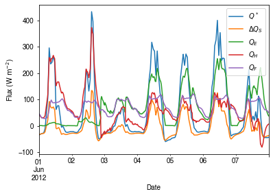
Quick look at the simulation results:
[22]:
ax_output = df_output_suews\
    .loc[grid]\
    .loc['2012 6 1':'2012 6 7',
         ['QN', 'QS', 'QE', 'QH', 'QF']]\
    .rename(columns=dict_var_disp)\
    .plot()
_ = ax_output.set_xlabel('Date')
_ = ax_output.set_ylabel('Flux ($ \mathrm{W \ m^{-2}}$)')
_ = ax_output.legend()
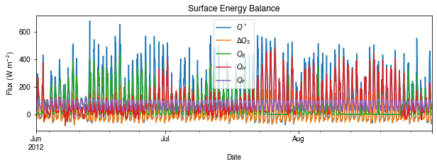
More examples
Below is a more complete example for examination of urban energy balance over the whole summer (June to August).
[23]:
# energy balance
ax_output = (
    df_output_suews.loc[grid]
    .loc["2012 6":"2012 8", ["QN", "QS", "QE", "QH", "QF"]]
    .rename(columns=dict_var_disp)
    .plot(figsize=(10, 3), title="Surface Energy Balance",)
)
_ = ax_output.set_xlabel("Date")
_ = ax_output.set_ylabel("Flux ($ \mathrm{W \ m^{-2}}$)")
_ = ax_output.legend()
Resampling
The suggested runtime/simulation frequency of SUEWS is 300 s, which usually results in a large output and may be over-weighted for storage and analysis. Also, you may feel an apparent slowdown in producing the above figure as a large amount of data were used for the plotting. To slim down the result size for analysis and output, we can resample the default output very easily.
[24]:
rsmp_1d = df_output_suews.loc[grid].resample("1d")
# daily mean values
df_1d_mean = rsmp_1d.mean()
# daily sum values
df_1d_sum = rsmp_1d.sum()
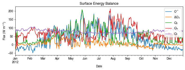
We can then re-examine the above energy balance at hourly scale and plotting will be significantly faster.
[25]:
# energy balance
ax_output = (
    df_1d_mean.loc[:, ["QN", "QS", "QE", "QH", "QF"]]
    .rename(columns=dict_var_disp)
    .plot(figsize=(10, 3), title="Surface Energy Balance",)
)
_ = ax_output.set_xlabel("Date")
_ = ax_output.set_ylabel("Flux ($ \mathrm{W \ m^{-2}}$)")
_ = ax_output.legend()
Then we use the hourly results for other analyses.
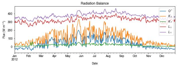
[26]:
# radiation balance
ax_output = (
    df_1d_mean.loc[:, ["QN", "Kdown", "Kup", "Ldown", "Lup"]]
    .rename(columns=dict_var_disp)
    .plot(figsize=(10, 3), title="Radiation Balance",)
)
_ = ax_output.set_xlabel("Date")
_ = ax_output.set_ylabel("Flux ($ \mathrm{W \ m^{-2}}$)")
_ = ax_output.legend()
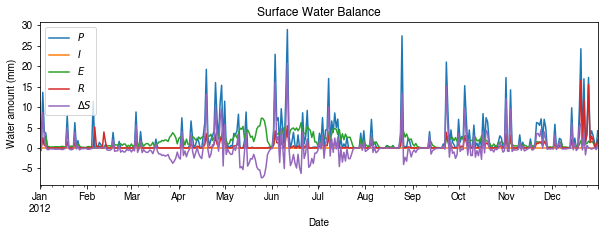
[27]:
# water balance
ax_output = (
    df_1d_sum.loc[:, ["Rain", "Irr", "Evap", "RO", "TotCh"]]
    .rename(columns=dict_var_disp)
    .plot(figsize=(10, 3), title="Surface Water Balance",)
)
_ = ax_output.set_xlabel("Date")
_ = ax_output.set_ylabel("Water amount (mm)")
_ = ax_output.legend()
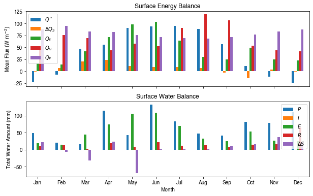
Get an overview of partitioning in energy and water balance at monthly scales:
[28]:
# get a monthly Resampler
df_plot = df_output_suews.loc[grid].copy()
df_plot.index = df_plot.index.set_names("Month")
rsmp_1M = df_plot.shift(-1).dropna(how="all").resample("1M", kind="period")
# mean values
df_1M_mean = rsmp_1M.mean()
# sum values
df_1M_sum = rsmp_1M.sum()
[29]:
# month names
name_mon = [x.strftime("%b") for x in rsmp_1M.groups]
# create subplots showing two panels together
fig, axes = plt.subplots(2, 1, sharex=True)
# surface energy balance
df_1M_mean.loc[:, ["QN", "QS", "QE", "QH", "QF"]].rename(columns=dict_var_disp).plot(
    ax=axes[0],  # specify the axis for plotting
    figsize=(10, 6),  # specify figure size
    title="Surface Energy Balance",
    kind="bar",
)
# surface water balance
df_1M_sum.loc[:, ["Rain", "Irr", "Evap", "RO", "TotCh"]].rename(
    columns=dict_var_disp
).plot(
    ax=axes[1],  # specify the axis for plotting
    title="Surface Water Balance",
    kind="bar",
)

# annotations
_ = axes[0].set_ylabel("Mean Flux ($ \mathrm{W \ m^{-2}}$)")
_ = axes[0].legend()
_ = axes[1].set_xlabel("Month")
_ = axes[1].set_ylabel("Total Water Amount (mm)")
_ = axes[1].xaxis.set_ticklabels(name_mon, rotation=0)
_ = axes[1].legend()
[29]:
<matplotlib.axes._subplots.AxesSubplot at 0x7fb081241128>
[29]:
<matplotlib.axes._subplots.AxesSubplot at 0x7fb0942eb5f8>
Output
The supy output can be saved as txt files for further analysis using supy function save_supy.
[30]:
df_output
[30]:
| group | SUEWS | ... | DailyState | |||||||||||||||||||
|---|---|---|---|---|---|---|---|---|---|---|---|---|---|---|---|---|---|---|---|---|---|---|
| var | Kdown | Kup | Ldown | Lup | Tsurf | QN | QF | QS | QH | QE | ... | DensSnow_Paved | DensSnow_Bldgs | DensSnow_EveTr | DensSnow_DecTr | DensSnow_Grass | DensSnow_BSoil | DensSnow_Water | a1 | a2 | a3 | |
| grid | datetime | |||||||||||||||||||||
| 1 | 2012-01-01 00:05:00 | 0.176667 | 0.021459 | 344.179805 | 371.680316 | 11.607207 | -27.345303 | 40.574001 | -5.886447 | 15.276915 | -7.777741 | ... | NaN | NaN | NaN | NaN | NaN | NaN | NaN | NaN | NaN | NaN |
| 2012-01-01 00:10:00 | 0.173333 | 0.046164 | 344.190048 | 372.637243 | 11.620000 | -28.320026 | 39.724283 | -1.013319 | -22.518257 | -81.748807 | ... | NaN | NaN | NaN | NaN | NaN | NaN | NaN | NaN | NaN | NaN | |
| 2012-01-01 00:15:00 | 0.170000 | 0.045271 | 344.200308 | 372.715137 | 11.635000 | -28.390100 | 38.874566 | -1.001900 | -23.450672 | -82.273388 | ... | NaN | NaN | NaN | NaN | NaN | NaN | NaN | NaN | NaN | NaN | |
| 2012-01-01 00:20:00 | 0.166667 | 0.044378 | 344.210586 | 372.793044 | 11.650000 | -28.460168 | 38.024849 | -0.989860 | -24.350304 | -82.818868 | ... | NaN | NaN | NaN | NaN | NaN | NaN | NaN | NaN | NaN | NaN | |
| 2012-01-01 00:25:00 | 0.163333 | 0.043485 | 344.220882 | 372.870963 | 11.665000 | -28.530232 | 37.175131 | -0.977988 | -25.191350 | -83.410146 | ... | NaN | NaN | NaN | NaN | NaN | NaN | NaN | NaN | NaN | NaN | |
| ... | ... | ... | ... | ... | ... | ... | ... | ... | ... | ... | ... | ... | ... | ... | ... | ... | ... | ... | ... | ... | ... | |
| 2012-12-31 23:35:00 | 0.000000 | 0.000000 | 330.263407 | 363.676342 | 10.140000 | -33.412935 | 53.348682 | -4.399144 | 2.559974 | 21.774918 | ... | NaN | NaN | NaN | NaN | NaN | NaN | NaN | NaN | NaN | NaN | |
| 2012-12-31 23:40:00 | 0.000000 | 0.000000 | 330.263407 | 363.676342 | 10.140000 | -33.412935 | 52.422737 | -4.397669 | 2.178582 | 21.228889 | ... | NaN | NaN | NaN | NaN | NaN | NaN | NaN | NaN | NaN | NaN | |
| 2012-12-31 23:45:00 | 0.000000 | 0.000000 | 330.263407 | 363.676342 | 10.140000 | -33.412935 | 51.496792 | -4.395831 | 1.797190 | 20.682498 | ... | NaN | NaN | NaN | NaN | NaN | NaN | NaN | NaN | NaN | NaN | |
| 2012-12-31 23:50:00 | 0.000000 | 0.000000 | 330.263407 | 363.676342 | 10.140000 | -33.412935 | 50.570847 | -4.393681 | 1.436708 | 20.114885 | ... | NaN | NaN | NaN | NaN | NaN | NaN | NaN | NaN | NaN | NaN | |
| 2012-12-31 23:55:00 | 0.000000 | 0.000000 | 330.263407 | 363.676342 | 10.140000 | -33.412935 | 46.174492 | -4.391264 | -0.234230 | 17.387051 | ... | 100.0 | 100.0 | 100.0 | 100.0 | 100.0 | 100.0 | 449.702073 | 0.36935 | 0.3242 | 8.0995 | |
105407 rows × 371 columns
[33]:
list_path_save = sp.save_supy(df_output, df_state_final,)
[32]:
for file_out in list_path_save:
    print(file_out.name)
1_2012_DailyState.txt
1_2012_SUEWS_60.txt
1_2012_snow_60.txt
1_2012_RSL_60.txt
1_2012_SOLWEIG_60.txt
df_state.csv