Set up SuPy for Your Own Site
This tutorial aims to demonstrate how to set up SuPy for your own site to model the surface energy balance (SEB).
Please note: SuPy is a Python-enhanced urban climate model with SUEWS, *Surface Urban Energy and Water Balance Scheme*, as its computation core.
We thus strongly recommend/encourage users to have a good understanding of SUEWS first before diving into the SuPy world.
In this tutorial, We will use an AmeriFlux site US-AR1 as example:
starting by preparation of input data, we show how to specify site characteristics and choose proper scheme options, then conduct simulations, finally provide some demo figures to help understand the simulation results.
A brief structure is as follows:
Boilerplate code
[1]:
import matplotlib.pyplot as plt
import supy as sp
import pandas as pd
import numpy as np
from pathlib import Path
%matplotlib inline
Prepare input data
Site-specific configuration of surface parameters
Given pandas.DataFrame as the core data structure of SuPy, all operations, including modification, output, demonstration, etc., on SuPy inputs (df_state_init and df_forcing) can be done using pandas-based functions/methods. Please see SuPy quickstart for methods to do so.
Below we will modify several key properties of the chosen site with appropriate values to run SuPy. First, we copy the df_state_init to have a new DataFrame for manipulation.
[2]:
df_state_init,df_forcing=sp.load_SampleData()
df_state_amf = df_state_init.copy()
2020-07-06 11:24:40,102 - SuPy - INFO - All cache cleared.
[3]:
# site identifier
name_site = 'US-AR1'
Details for determining the proper values of selected physical parameters can be found here.
location
[4]:
# latitude
df_state_amf.loc[:, 'lat'] = 41.37
# longitude
df_state_amf.loc[:, 'lng'] = -106.24
# altitude
df_state_amf.loc[:, 'alt'] = 611.
land cover fraction
[5]:
# view the surface fraction variable: `sfr`
df_state_amf.loc[:, 'sfr'] = 0
df_state_amf.loc[:, ('sfr', '(4,)')] = 1
df_state_amf.loc[:, 'sfr']
[5]:
| ind_dim | (0,) | (1,) | (2,) | (3,) | (4,) | (5,) | (6,) |
|---|---|---|---|---|---|---|---|
| grid | |||||||
| 1 | 0.0 | 0.0 | 0.0 | 0.0 | 1.0 | 0.0 | 0.0 |
albedo
[6]:
# we only set values for grass as the modelled site has a single land cover type: grass.
df_state_amf.albmax_grass = 0.19
df_state_amf.albmin_grass = 0.14
[7]:
# initial albedo value
df_state_amf.loc[:, 'albgrass_id'] = 0.14
LAI/phenology
[8]:
df_state_amf.filter(like='lai')
[8]:
| var | laimax | laimin | laipower | laitype | laicalcyes | lai_id | |||||||||||||||
|---|---|---|---|---|---|---|---|---|---|---|---|---|---|---|---|---|---|---|---|---|---|
| ind_dim | (0,) | (1,) | (2,) | (0,) | (1,) | (2,) | (0, 0) | (0, 1) | (0, 2) | (1, 0) | ... | (3, 0) | (3, 1) | (3, 2) | (0,) | (1,) | (2,) | 0 | (0,) | (1,) | (2,) |
| grid | |||||||||||||||||||||
| 1 | 5.1 | 5.5 | 5.9 | 4.0 | 1.0 | 1.6 | 0.04 | 0.04 | 0.04 | 0.001 | ... | 0.0015 | 0.0015 | 0.0015 | 1.0 | 1.0 | 1.0 | 1 | 4.0 | 1.0 | 1.6 |
1 rows × 25 columns
[9]:
# properties to control vegetation phenology
# you can skip the details for and just set them as provided below

# LAI paramters
df_state_amf.loc[:, ('laimax', '(2,)')] = 1
df_state_amf.loc[:, ('laimin', '(2,)')] = 0.2
# initial LAI
df_state_amf.loc[:, ('lai_id', '(2,)')] = 0.2

# BaseT
df_state_amf.loc[:, ('baset', '(2,)')] = 5
# BaseTe
df_state_amf.loc[:, ('basete', '(2,)')] = 20

# SDDFull
df_state_amf.loc[:, ('sddfull', '(2,)')] = -1000
# GDDFull
df_state_amf.loc[:, ('gddfull', '(2,)')] = 1000
surface resistance
[10]:
# parameters to model surface resistance
df_state_amf.maxconductance = 18.7
df_state_amf.g1 = 1
df_state_amf.g2 = 104.215
df_state_amf.g3 = 0.424
df_state_amf.g4 = 0.814
df_state_amf.g5 = 36.945
df_state_amf.g6 = 0.025
measurement height
[11]:
# height where forcing variables are measured/collected
df_state_amf.z = 2.84
urban feature
[12]:
# disable anthropogenic heat by setting zero population
df_state_amf.popdensdaytime = 0
df_state_amf.popdensnighttime = 0
check df_state
[13]:
# this procedure is to double-check proper values are set in `df_state_amf`
sp.check_state(df_state_amf)
2020-07-06 11:24:43,372 - SuPy - INFO - SuPy is validating `df_state`...
2020-07-06 11:24:43,574 - SuPy - INFO - All checks for `df_state` passed!
prepare forcing conditions
Here we use the SuPy utility function read_forcing to read in forcing data from an external file in the format of SUEWS input. Also note, this read_forcing utility will also resample the forcing data to a proper temporal resolution to run SuPy/SUEWS, which is usually 5 min (300 s).
load and resample forcing data
UMEP workshop users: please note the AMF file path might be DIFFERENT from yours; please set it to the location where your downloaded file is placed.
[15]:
# load forcing data from an external file and resample to a resolution of 300 s.
# Note this dataset has been gap-filled.
df_forcing_amf = sp.util.read_forcing("data/US-AR1_2010_data_60.txt", tstep_mod=300)

# this procedure is to double-check proper forcing values are set in `df_forcing_amf`
_ = sp.check_forcing(df_forcing_amf)
2020-07-06 11:24:44,453 - SuPy - INFO - SuPy is validating `df_forcing`...
2020-07-06 11:24:46,299 - SuPy - ERROR - Issues found in `df_forcing`:
`kdown` should be between [0, 1400] but `-1.298` is found at 2010-01-01 00:05:00
The checker detected invalid values in variable kdown: negative incoming solar radiation is found. We then need to fix this as follows:
[16]:
# modify invalid values
df_forcing_amf.kdown = df_forcing_amf.kdown.where(df_forcing_amf.kdown > 0, 0)
[17]:
# check `df_forcing` again
_ = sp.check_forcing(df_forcing_amf)
2020-07-06 11:24:46,312 - SuPy - INFO - SuPy is validating `df_forcing`...
2020-07-06 11:24:48,523 - SuPy - INFO - All checks for `df_forcing` passed!
examine forcing data
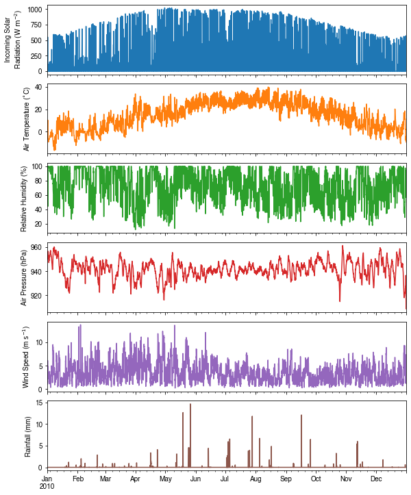
We can examine the forcing data:
[18]:
list_var_forcing = [
    "kdown",
    "Tair",
    "RH",
    "pres",
    "U",
    "rain",
]
dict_var_label = {
    "kdown": "Incoming Solar\n Radiation ($ \mathrm{W \ m^{-2}}$)",
    "Tair": "Air Temperature ($^{\circ}}$C)",
    "RH": r"Relative Humidity (%)",
    "pres": "Air Pressure (hPa)",
    "rain": "Rainfall (mm)",
    "U": "Wind Speed (m $\mathrm{s^{-1}}$)",
}
df_plot_forcing_x = (
    df_forcing_amf.loc[:, list_var_forcing].copy().shift(-1).dropna(how="any")
)
df_plot_forcing = df_plot_forcing_x.resample("1h").mean()
df_plot_forcing["rain"] = df_plot_forcing_x["rain"].resample("1h").sum()

axes = df_plot_forcing.plot(subplots=True, figsize=(8, 12), legend=False,)
fig = axes[0].figure
fig.tight_layout()
fig.autofmt_xdate(bottom=0.2, rotation=0, ha="center")
for ax, var in zip(axes, list_var_forcing):
    _ = ax.set_ylabel(dict_var_label[var])
Run simulations
Once met-forcing (via df_forcing_amf) and initial conditions (via df_state_amf) are loaded in, we call sp.run_supy to conduct a SUEWS simulation, which will return two pandas DataFrames: df_output and df_state_final.
[19]:
df_output, df_state_final = sp.run_supy(df_forcing_amf, df_state_amf)
2020-07-06 11:24:51,973 - SuPy - INFO - ====================
2020-07-06 11:24:51,974 - SuPy - INFO - Simulation period:
2020-07-06 11:24:51,975 - SuPy - INFO -   Start: 2010-01-01 00:05:00
2020-07-06 11:24:51,975 - SuPy - INFO -   End: 2011-01-01 00:00:00
2020-07-06 11:24:51,976 - SuPy - INFO -
2020-07-06 11:24:51,977 - SuPy - INFO - No. of grids: 1
2020-07-06 11:24:51,977 - SuPy - INFO - SuPy is running in serial mode
2020-07-06 11:25:01,975 - SuPy - INFO - Execution time: 10.0 s
2020-07-06 11:25:01,976 - SuPy - INFO - ====================
df_output
df_output is an ensemble output collection of major SUEWS output groups, including:
SUEWS: the essential SUEWS output variables
DailyState: variables of daily state information
snow: snow output variables (effective when
snowuse = 1set indf_state_init)RSL: profile of air temperature, humidity and wind speed within roughness sub-layer.
Detailed description of variables in df_output refers to SuPy output
[20]:
df_output.columns.levels[0]
[20]:
Index(['SUEWS', 'snow', 'RSL', 'SOLWEIG', 'DailyState'], dtype='object', name='group')
df_state_final
df_state_final is a DataFrame for holding:
all model states if
save_stateis set toTruewhen callingsp.run_supy(supymay run significantly slower for a large simulations);or, only the final state if
save_stateis set toFalse(the default setting) in which modesupyhas a similar performance as the standalone compiled SUEWS executable.
Entries in df_state_final have the same data structure as df_state_init and can thus be used for other SUEWS simulations staring at the timestamp as in df_state_final.
Detailed description of variables in df_state_final refers to SuPy output
[21]:
df_state_final.T.head()
[21]:
| datetime | 2010-01-01 00:05:00 | 2011-01-01 00:05:00 | |
|---|---|---|---|
| grid | 1 | 1 | |
| var | ind_dim | ||
| ah_min | (0,) | 15.0 | 15.0 |
| (1,) | 15.0 | 15.0 | |
| ah_slope_cooling | (0,) | 2.7 | 2.7 |
| (1,) | 2.7 | 2.7 | |
| ah_slope_heating | (0,) | 2.7 | 2.7 |
Examine results
Thanks to the functionality inherited from pandas and other packages under the PyData stack, compared with the standard SUEWS simulation workflow, supy enables more convenient examination of SUEWS results by statistics calculation, resampling, plotting (and many more).
Ouptut structure
df_output is organised with MultiIndex (grid,timestamp) and (group,varaible) as index and columns, respectively.
[22]:
df_output.head()
[22]:
| group | SUEWS | ... | DailyState | |||||||||||||||||||
|---|---|---|---|---|---|---|---|---|---|---|---|---|---|---|---|---|---|---|---|---|---|---|
| var | Kdown | Kup | Ldown | Lup | Tsurf | QN | QF | QS | QH | QE | ... | DensSnow_Paved | DensSnow_Bldgs | DensSnow_EveTr | DensSnow_DecTr | DensSnow_Grass | DensSnow_BSoil | DensSnow_Water | a1 | a2 | a3 | |
| grid | datetime | |||||||||||||||||||||
| 1 | 2010-01-01 00:05:00 | 0.0 | 0.0 | 265.492652 | 305.638434 | -1.593 | -40.145783 | 0.0 | -9.668746 | -24.387976 | 1.284400 | ... | NaN | NaN | NaN | NaN | NaN | NaN | NaN | NaN | NaN | NaN |
| 2010-01-01 00:10:00 | 0.0 | 0.0 | 265.492652 | 305.638434 | -1.593 | -40.145783 | 0.0 | -9.424108 | -6.676973 | 1.618190 | ... | NaN | NaN | NaN | NaN | NaN | NaN | NaN | NaN | NaN | NaN | |
| 2010-01-01 00:15:00 | 0.0 | 0.0 | 265.492652 | 307.825865 | -1.593 | -42.333213 | 0.0 | -0.545992 | 16.458627 | 11.833592 | ... | NaN | NaN | NaN | NaN | NaN | NaN | NaN | NaN | NaN | NaN | |
| 2010-01-01 00:20:00 | 0.0 | 0.0 | 265.492652 | 307.825865 | -1.593 | -42.333213 | 0.0 | -0.536225 | 15.988621 | 11.830741 | ... | NaN | NaN | NaN | NaN | NaN | NaN | NaN | NaN | NaN | NaN | |
| 2010-01-01 00:25:00 | 0.0 | 0.0 | 265.492652 | 307.825865 | -1.593 | -42.333213 | 0.0 | -0.525680 | 15.537087 | 11.827934 | ... | NaN | NaN | NaN | NaN | NaN | NaN | NaN | NaN | NaN | NaN | |
5 rows × 371 columns
Here we demonstrate several typical scenarios for SUEWS results examination.
The essential SUEWS output collection is extracted as a separate variable for easier processing in the following sections. More advanced slicing techniques are available in pandas documentation.
[23]:
grid = df_state_amf.index[0]
df_output_suews = df_output.loc[grid, 'SUEWS']
Statistics Calculation
We can use .describe() method for a quick overview of the key surface energy balance budgets.
[24]:
df_output_suews.loc[:, ['QN', 'QS', 'QH', 'QE', 'QF']].describe()
[24]:
| var | QN | QS | QH | QE | QF |
|---|---|---|---|---|---|
| count | 105120.000000 | 105120.000000 | 105120.000000 | 105120.000000 | 105120.0 |
| mean | 118.207887 | 19.047648 | 38.349672 | 62.790798 | 0.0 |
| std | 214.335328 | 61.955598 | 85.050755 | 112.585643 | 0.0 |
| min | -104.566267 | -81.170768 | -212.925432 | -15.483971 | 0.0 |
| 25% | -33.437969 | -23.174678 | -15.992876 | 0.341017 | 0.0 |
| 50% | -1.894385 | -2.603727 | 9.862241 | 3.042328 | 0.0 |
| 75% | 248.960723 | 52.299898 | 68.130871 | 65.272384 | 0.0 |
| max | 749.868243 | 218.450452 | 414.514498 | 559.472107 | 0.0 |
Plotting
Basic example
Plotting is very straightforward via the .plot method bounded with pandas.DataFrame. Note the usage of loc for to slices of the output DataFrame.
[25]:
# a dict for better display variable names
dict_var_disp = {
    "QN": "$Q^*$",
    "QS": r"$\Delta Q_S$",
    "QE": "$Q_E$",
    "QH": "$Q_H$",
    "QF": "$Q_F$",
    "Kdown": r"$K_{\downarrow}$",
    "Kup": r"$K_{\uparrow}$",
    "Ldown": r"$L_{\downarrow}$",
    "Lup": r"$L_{\uparrow}$",
    "Rain": "$P$",
    "Irr": "$I$",
    "Evap": "$E$",
    "RO": "$R$",
    "TotCh": "$\Delta S$",
}
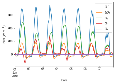
Peek at the simulation results:
[26]:
grid = df_state_init.index[0]
[27]:
ax_output = (
    df_output_suews.loc["2010-06-01":"2010-06-07", ["QN", "QS", "QE", "QH", "QF"]]
    .rename(columns=dict_var_disp)
    .plot()
)
_ = ax_output.set_xlabel("Date")
_ = ax_output.set_ylabel("Flux ($ \mathrm{W \ m^{-2}}$)")
_ = ax_output.legend()
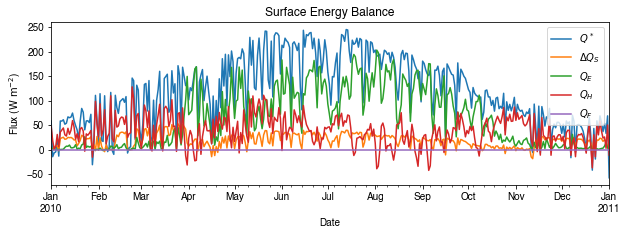
Plotting after resampling
The suggested runtime/simulation frequency of SUEWS is 300 s, which usually results in a large output and may be over-weighted for storage and analysis. Also, you may feel an apparent slowdown in producing the above figure as a large amount of data were used for the plotting. To slim down the result size for analysis and output, we can resample the default output very easily.
[28]:
rsmp_1d = df_output_suews.resample("1d")
# daily mean values
df_1d_mean = rsmp_1d.mean()
# daily sum values
df_1d_sum = rsmp_1d.sum()
We can then re-examine the above energy balance at hourly scale and plotting will be significantly faster.
[29]:
# energy balance
ax_output = (
    df_1d_mean.loc[:, ["QN", "QS", "QE", "QH", "QF"]]
    .rename(columns=dict_var_disp)
    .plot(figsize=(10, 3), title="Surface Energy Balance",)
)
_ = ax_output.set_xlabel("Date")
_ = ax_output.set_ylabel("Flux ($ \mathrm{W \ m^{-2}}$)")
_ = ax_output.legend()
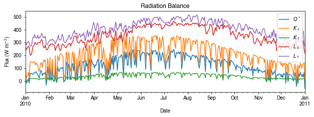
Then we use the hourly results for other analyses.
[30]:
# radiation balance
ax_output = (
    df_1d_mean.loc[:, ["QN", "Kdown", "Kup", "Ldown", "Lup"]]
    .rename(columns=dict_var_disp)
    .plot(figsize=(10, 3), title="Radiation Balance",)
)
_ = ax_output.set_xlabel("Date")
_ = ax_output.set_ylabel("Flux ($ \mathrm{W \ m^{-2}}$)")
_ = ax_output.legend()
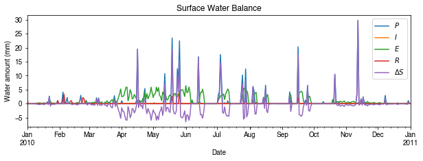
[31]:
# water balance
ax_output = (
    df_1d_sum.loc[:, ["Rain", "Irr", "Evap", "RO", "TotCh"]]
    .rename(columns=dict_var_disp)
    .plot(figsize=(10, 3), title="Surface Water Balance",)
)
_ = ax_output.set_xlabel("Date")
_ = ax_output.set_ylabel("Water amount (mm)")
_ = ax_output.legend()
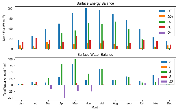
Get an overview of partitioning in energy and water balance at monthly scales:
[32]:
# get a monthly Resampler
df_plot = df_output_suews.copy()
df_plot.index = df_plot.index.set_names("Month")
rsmp_1M = df_plot.shift(-1).dropna(how="all").resample("1M", kind="period")
# mean values
df_1M_mean = rsmp_1M.mean()
# sum values
df_1M_sum = rsmp_1M.sum()
[33]:
# month names
name_mon = [x.strftime("%b") for x in rsmp_1M.groups]
# create subplots showing two panels together
fig, axes = plt.subplots(2, 1, sharex=True)
# surface energy balance
_ = (
    df_1M_mean.loc[:, ["QN", "QS", "QE", "QH", "QF"]]
    .rename(columns=dict_var_disp)
    .plot(
        ax=axes[0],  # specify the axis for plotting
        figsize=(10, 6),  # specify figure size
        title="Surface Energy Balance",
        kind="bar",
    )
)
# surface water balance
_ = (
    df_1M_sum.loc[:, ["Rain", "Irr", "Evap", "RO", "TotCh"]]
    .rename(columns=dict_var_disp)
    .plot(
        ax=axes[1],  # specify the axis for plotting
        title="Surface Water Balance",
        kind="bar",
    )
)

# annotations
_ = axes[0].set_ylabel("Mean Flux ($ \mathrm{W \ m^{-2}}$)")
_ = axes[0].legend()
_ = axes[1].set_xlabel("Month")
_ = axes[1].set_ylabel("Total Water Amount (mm)")
_ = axes[1].xaxis.set_ticklabels(name_mon, rotation=0)
_ = axes[1].legend()
Save results to external files
The supy output can be saved as txt files for further analysis using supy function save_supy.
[34]:
list_path_save = sp.save_supy(df_output, df_state_final)
[35]:
for file_out in list_path_save:
    print(file_out.name)
1_2010_DailyState.txt
1_2010_SUEWS_60.txt
1_2010_snow_60.txt
1_2010_RSL_60.txt
1_2010_SOLWEIG_60.txt
df_state.csv
More explorations into simulation results
In this section, we will use the simulation results to explore more features revealed by SuPy/SUEWS simulations but unavailable in your simple model.
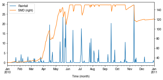
Dynamics in rainfall and soil moisture deficit (SMD)
[36]:
df_dailystate = (
    df_output.loc[grid, "DailyState"].dropna(how="all").resample("1d").mean()
)
[37]:
# daily rainfall
ser_p = df_dailystate.P_day.rename("Rainfall")
ser_smd = df_output_suews.SMD
ser_smd_dmax = ser_smd.resample("1d").max().rename("SMD")

ax = pd.concat([ser_p, ser_smd_dmax], axis=1).plot(secondary_y="SMD", figsize=(9, 4))
_ = ax.set_xlabel("Time (month)")
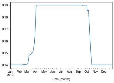
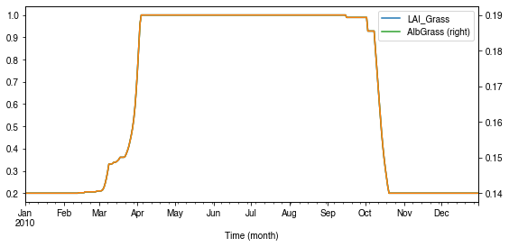
Variability in albedo
How does albedo change over time?
[38]:
ser_alb = df_dailystate.AlbGrass
ax = ser_alb.plot()
_ = ax.set_xlabel("Time (month)")
How is albedo associated with vegetation phenology?
[39]:
ser_lai = df_dailystate.LAI_Grass
pd.concat([ser_lai, ser_alb], axis=1).plot(secondary_y="AlbGrass", figsize=(9, 4))
ax = ser_lai.plot()
_ = ax.set_xlabel("Time (month)")
[39]:
<matplotlib.axes._subplots.AxesSubplot at 0x7f8969449978>
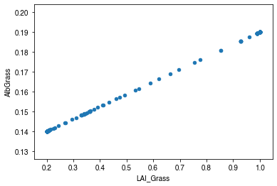
[40]:
ax_alb_lai = df_dailystate[["LAI_Grass", "AlbGrass"]].plot.scatter(
    x="LAI_Grass", y="AlbGrass",
)
ax_alb_lai.set_aspect("auto")
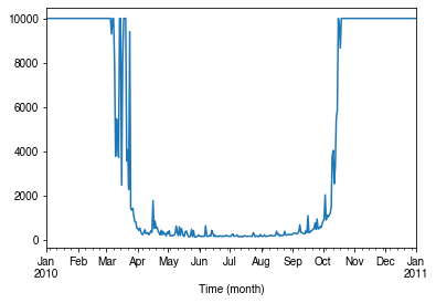
Variability in surface resistance
How does surface resistance vary over time?
[41]:
ser_rs = df_output_suews.RS
intra-annual
[42]:
ax = ser_rs.resample("1d").median().plot()
_ = ax.set_xlabel("Time (month)")
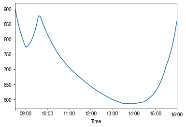
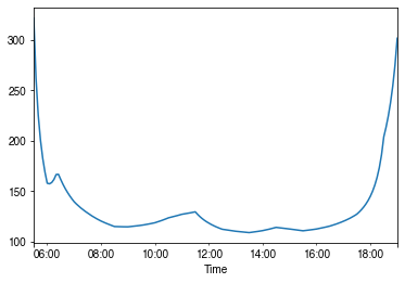
intra-daily
[43]:
# a winter day
ax = ser_rs.loc["2010-01-22"].between_time("0830", "1600").plot()
_ = ax.set_xlabel("Time")
[44]:
# a summer day
ax = ser_rs.loc["2010-07-01"].between_time("0530", "1900").plot()
_ = ax.set_xlabel("Time")
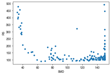
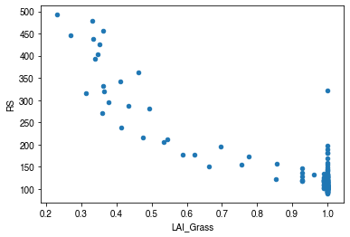
How is surface resistance associated with other surface properties?
[45]:
# SMD
ser_smd = df_output_suews.SMD
df_x = (
    pd.concat([ser_smd, ser_rs], axis=1)
    .between_time("1000", "1600")
    .resample("1d")
    .mean()
)
df_x = df_x.loc[df_x.RS < 500]
_ = df_x.plot.scatter(x="SMD", y="RS",)
[46]:
# LAI
df_x = pd.concat(
    [ser_lai, ser_rs.between_time("1000", "1600").resample("1d").mean()], axis=1
)
df_x = df_x.loc[df_x.RS < 500]
_ = df_x.plot.scatter(x="LAI_Grass", y="RS",)
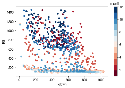
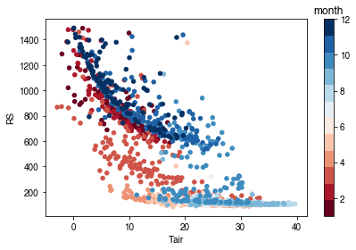
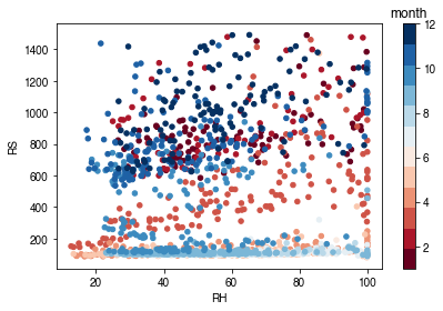
How is surface resistance dependent on meteorological conditions?
[47]:
cmap_sel = plt.cm.get_cmap('RdBu', 12)
[48]:
# solar radiation
# colour by season
ser_kdown = df_forcing_amf.kdown
df_x = pd.concat([ser_kdown, ser_rs], axis=1).between_time('1000', '1600')
df_x = df_x.loc[df_x.RS < 1500]
df_plot = df_x.iloc[::20]
ax = df_plot.plot.scatter(x='kdown',
                          y='RS',
                          c=df_plot.index.month,
                          cmap=cmap_sel,
                          sharex=False)
fig = ax.figure
_ = fig.axes[1].set_title('month')
fig.tight_layout()
[49]:
# air temperature
ser_ta = df_forcing_amf.Tair
df_x = pd.concat([ser_ta, ser_rs], axis=1).between_time('1000', '1600')
df_x = df_x.loc[df_x.RS < 1500]
df_plot = df_x.iloc[::15]
ax = df_plot.plot.scatter(x='Tair',
                          y='RS',
                          c=df_plot.index.month,
                          cmap=cmap_sel,
                          sharex=False)
fig = ax.figure
_ = fig.axes[1].set_title('month')
fig.tight_layout()
[50]:
# air humidity
ser_rh = df_forcing_amf.RH
df_x = pd.concat([ser_rh, ser_rs], axis=1).between_time('1000', '1600')
df_x = df_x.loc[df_x.RS < 1500]
df_plot = df_x.iloc[::15]
ax = df_plot.plot.scatter(x='RH',
                          y='RS',
                          c=df_plot.index.month,
                          cmap=cmap_sel,
                          sharex=False)
fig = ax.figure
_ = fig.axes[1].set_title('month')
fig.tight_layout()
Task:
Based on the above plots showing RS vs. met. conditions, explore these relationships again at the intra-daily scales.